Image Classification using CNNs and ResNets in PyTorch

Part 5 of "PyTorch: Zero to GANs"

This post is the fifth in a series of tutorials on building deep learning models with PyTorch, an open source neural networks library. Check out the full series:

1. PyTorch Basics: Tensors & Gradients
2. Linear Regression & Gradient Descent
3. Image Classfication using Logistic Regression
4. Training Deep Neural Networks on a GPU
5. Image Classification using CNNs (this notebook)
6. Generative Adverserial Networks (GANs)

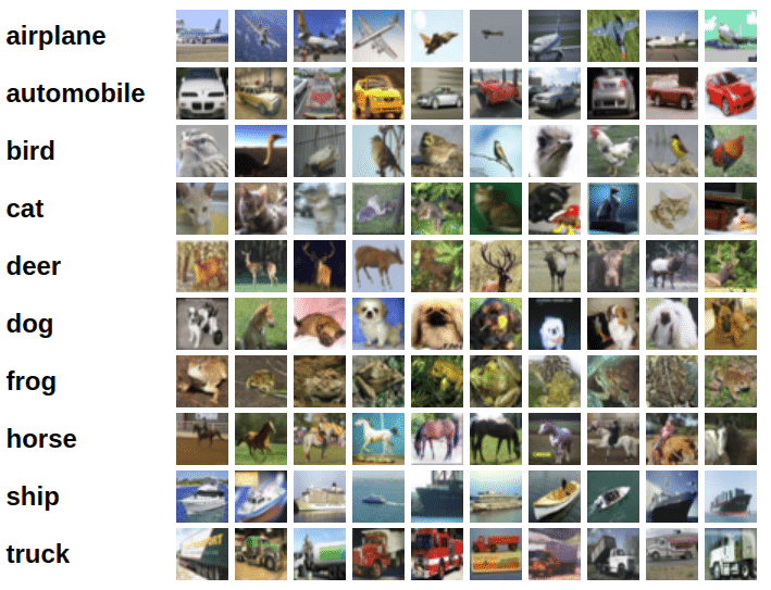
In the previous tutorial, we trained a feedfoward neural networks with a single hidden layer to classify handwritten digits from the MNIST dataset with over 97% accuracy. For this tutorial, we'll use the CIFAR10 dataset, which consists of 60000 32x32 px colour images in 10 classes. Here are some sample images from the dataset:

System Setup

This notebook is hosted on Jovian.ml, a platform for sharing data science projects. If you want to follow along and run the code as you read, you can choose the "Run on Kaggle" option from the "Run" dropdown above. Otherwise, to run the code on your machine, you can clone the notebook, install the required dependencies using conda, and start Juptyer by running the following commands:

pip install jovian --upgrade   # Install the jovian library 
jovian clone 05-cifar10-cnn    # Download notebook & dependencies
cd 05-cifar10-cnn              # Enter the created directory 
conda env update               # Install the dependencies
conda activate 05-cifar10-cnn  # Activate virtual env
jupyter notebook               # Start Jupyter

On older versions of conda, you might need to run source activate 05-cifar10-cnn to activate the environment. For a more detailed explanation of the above steps, check out the System setup section in the first notebook.

Before you start executing the code below, you may want to clear the cell outputs by selecting "Kernel > Restart and Clear Output" from the Jupyter notebook menu bar, to avoid confusion.

Exploring the Data

We'll download the images in PNG format from this page, using some helper functions from the torchvision and tarfile packages.

The dataset is extracted to the directory data/cifar10. It contains 2 folders train and test, containing the training set (50000 images) and test set (10000 images) respectively. Each of them contains 10 folders, one for each class of images. Let's verify this using os.listdir.

Let's look inside a couple of folders, one from the training set and another from the test set. As an exercise, you can verify that that there are an equal number of images for each class, 5000 in the training set and 1000 in the test set.

The above directory structure (one folder per class) is used by many computer vision datasets, and most deep learning libraries provide utilites for working with such datasets. We can use the ImageFolder class from torchvision to load the data as PyTorch tensors.

Let's look at a sample element from the training dataset. Each element is a tuple, containing a image tensor and a label. Since the data consists of 32x32 px color images with 3 channels (RGB), each image tensor has the shape (3, 32, 32).

The list of classes is stored in the .classes property of the dataset. The numeric label for each element corresponds to index of the element's label in the list of classes.

We can view the image using matplotlib, but we need to change the tensor dimensions to (32,32,3). Let's create a helper function to display an image and its label.

Let's look at a couple of images from the dataset. As you can tell, the 32x32px images are quite difficult to identify, even for the human eye. Try changing the indices below to view different images.

Before continuing, let's save our work using the jovian python library.

jovian.commit uploads the notebook to your Jovian.ml account, captures the Python environment and creates a sharable link for your notebook as shown above. You can use this link to share your work and let anyone run it online or reproduce it with the jovian clone command.

Training and Validation Datasets

While building real world machine learning models, it is quite common to split the dataset into 3 parts:

1. Training set - used to train the model i.e. compute the loss and adjust the weights of the model using gradient descent.
2. Validation set - used to evaluate the model while training, adjust hyperparameters (learning rate etc.) and pick the best version of the model.
3. Test set - used to compare different models, or different types of modeling approaches, and report the final accuracy of the model.

Since there's no predefined validation set, we can set aside a small portion of the training set to be used as the validation set. Let's define a function that randomly picks a given fraction of the element indices for creating the validation set. We'll also pass a random seed into the function, so we can recreate the same training/validation split in future runs.

The jovian library also provides a simple API for recording important parameters related to the dataset, model training, results etc. for easy reference and comparison between multiple experiments. Let's record dataset_url, val_pct and rand_seed using jovian.log_dataset.

We have randomly shuffled the indices, and selected a small portion ( 20% ) to serve as the validation set. To process our data in small batches, we can now create PyTorch data loaders for each of these using a SubsetRandomSampler, which samples elements randomly from a given list of indices, while greating batches of data.

We can look at batches of images from the dataset using the make_grid method from torchvision. Each time the following code is run, we get a different bach, since the sampler shuffles the indices before creating batches.

Once again, let's save and commit our work using jovian before proceeding further.

After the first commit, all subsequent commits record a new version of the notebook within the same Jovian project. You can use jovian.commit to version Jupyter notebooks (instead of doing File > Save As), and keep your data science projects organized. Also check out the Records tab on the project page to see how the information logged using jovian.log_dataset appears on the UI.

Defining the Model (Convolutional Neural Network)

In our previous tutorial, we defined a deep neural network with fully-connected layers using nn.Linear. For this tutorial however, we will use a convolutional neural network, using the nn.Conv2d class from PyTorch.

The 2D convolution is a fairly simple operation at heart: you start with a kernel, which is simply a small matrix of weights. This kernel “slides” over the 2D input data, performing an elementwise multiplication with the part of the input it is currently on, and then summing up the results into a single output pixel. - Source

I highly recommend checking out the following articles if want to gain a better understanding of convolutions:

1. Intuitively understanding Convolutions for Deep Learning by Irhum Shafkat
2. Convolutions in Depth by Sylvian Gugger (this article implements convolutions from scratch)

There are certain advantages offered by convolutional layers when working with image data:

• Fewer parameters: A small set of parameters (the kernel) is used to calculate outputs of the entire image, so the model has much fewer parameters compared to a fully connected layer.
• Sparsity of connections: In each layer, each output element only depends on a small number of input elements, which makes the forward and backward passes more efficient.
• Parameter sharing and spatial invariance: The features learned by a kernel in one part of the image can be used to detect similar pattern in a different part of another image.

We will also use a max-pooling layers to progressively decrease the height & width of the output tensors from each convolutional layer.

Before we define the entire model, let's look at how a single convolutional layer followed by a max-pooling layer operates on the data.

Refer to Sylvian's post for an explanation of kernel_size, stride and padding.

The Conv2d layer transforms a 3-channel image to a 16-channel feature map, and the MaxPool2d layer halves the height and width. The feature map gets smaller as we add more layers, until we are finally left with a n x 1 x 1 feature map (where n is the no. of channels), which can be flattened into a vector. We can then add a fully connected layer at the end to get vector of size 10 for each image.

Let's verify that the model produces the expected output on a batch of training data. The 10 outputs for each image can be interpreted as probabilities for the 10 target classes (after applying softmax), and the class with the highest probability is chosen as the label predicted by the model for the input image. Check out Part 3 (logistic regression) for a more detailed discussion on interpeting the outputs, applying softmax and identifying the predicted labels.

To seamlessly use a GPU, if one is available, we define a couple of helper functions (get_default_device & to_device) and a helper class DeviceDataLoader to move our model & data to the GPU as required. These are described in more detail in the previous tutorial.

Based on where you're running this notebook, your default device could be a CPU (torch.device('cpu')) or a GPU (torch.device('cuda'))

We can now wrap our training and validation data loaders using DeviceDataLoader for automatically transferring batches of data to the GPU (if available), and use to_device to move our model to the GPU (if available).

Once again, let's save and commit the notebook before we proceed further.

Training the Model

As in the previous tutorials, we can use cross entropy as the loss function and accuracy as the evaluation metric for our model. The training loop is also identical, so we can reuse the loss_batch, evaluate and fit functions from the previous tutorial.

The loss_batch function calculates the loss and metric value for a batch of data, and optionally performs gradient descent if an optimizer is provided.

The evaluate function calculates the overall loss (and a metric, if provided) for the validation set.

The fit function (from the previous tutorial) contains the actual training loop: it sets up an optimizer, trains the model using the training set, then evaluates it on the validation set, then logs the losses, metrics etc. and repeats the process for the given number of epochs.

There's one important addition though: We invoke model.train() before training the model and model.eval() before evaluating it on the validation set. We'll discover what these methods do when we discuss regularization.

We also define an accuracy function which calculates the overall accuracy of the model on an entire batch of outputs, so that we can use it as a metric in fit.

Before we train the model, let's see how it performs on the validation set with the initial set of parameters.

The initial accuracy is around 10%, which is what one might expect from a randomly intialized model (since it has a 1 in 10 chance of getting a label right by guessing randomly).

We'll use the following hyperparmeters (learning rate, no. of epochs, batch_size etc.) to train our model. As an exercise, you can try changing these to see if you have achieve a higher accuracy in a shorter time.

It's important to record the hyperparameters of every experiment you do, to replicate it later and compare it against other experiments. We can record them using jovian.log_hyperparams.

Just as we have recorded the hyperparameters, we can also record the final metrics achieved by the model using jovian.log_metrics for reference, analysis and comparison.

We can also plot the valdation set accuracies to study how the model improves over time.

Our model reaches an accuracy of around 55%, and by looking at the graph, it seems unlikely that the model will achieve an accuracy higher than 65% even after training for a long time. This suggests that we might need to use a more powerful model to catpure the relationship between the images and the labels more accurately. This can be done by adding more convolutional layers to our model, or incrasing the no. of channels in each convolutional layer.

We can also plot the training and validation losses to study the trend.

Both the training and validation losses seem to decrease over time. However, if you train the model for long enough, you will notice that the training loss continues to decrease, while the validation loss stops decreasing, and even starts to increase after a certain point!

This phenomenon is called overfitting, and it is the no. 1 why many machine learning models give rather terrible results on real-world data. It happens because the model, in an attempt to minimize the loss, starts to learn patters are are unique to the training data, sometimes even memorizing specific training examples. Because of this, the model does not generalize well to previously unseen data.

Following are some common stragegies for avoiding overfitting:

• Gathering and generating more training data, or adding noise to it
• Using regularization techniques like batch normalization & dropout
• Early stopping of model's training, when validation loss starts to increase

We will cover these topics in more detail in the next tutorial in this series, and learn how we can reach an accuracy of over 90% by making minor but important changes to our model.

Before continuing, let us save our work to the cloud using jovian.commit.

When you try different experiments (by chaging the learning rate, batch size, optimizer etc.) and record hyperparameters and metrics with each version of your notebook, you can use the Compare view on the project page to analyze which approaches are working well and which ones aren't. You sort/filter by accuracy, loss etc., add notes for each version and even invite collaborators to contribute to your project with their own experiments.

Testing with individual images

While we have been tracking the overall accuracy of a model so far, it's also a good idea to look at model's results on some sample images. Let's test out our model with some images from the predefined test dataset of 10000 images. We begin by creating a test dataset using the ImageFolder class.

Let's define a helper function predict_image, which returns the predicted label for a single image tensor.

Identifying where our model performs poorly can help us improve the model, by collecting more training data, increasing/decreasing the complexity of the model, and changing the hypeparameters.

As a final step, let's also look at the overall loss and accuracy of the model on the test set, and record using jovian. We expect these values to be similar to those for the validation set. If not, we might need a better validation set that has similar data and distribution as the test set (which often comes from real world data).

Saving and loading the model

Since we've trained our model for a long time and achieved a resonable accuracy, it would be a good idea to save the weights of the model to disk, so that we can reuse the model later and avoid retraining from scratch. Here's how you can save the model.

The .state_dict method returns an OrderedDict containing all the weights and bias matrices mapped to the right attributes of the model. To load the model weights, we can redefine the model with the same structure, and use the .load_state_dict method.

Just as a sanity check, let's verify that this model has the same loss and accuracy on the test set as before.

Let's make one final commit using jovian, but this time, we will also attach the weights file as an output of our experiment, for future reference and sharing.

Check out the Files tab on the project page to view or download the trained model weights. You can also download all the files together using the Download Zip option in the Clone dropdown.

Data science work is often fragmented across many different platforms (Git for code, Dropbox/S3 for datasets & artifacts, spreadsheets for hyperparameters, metrics etc.) which can make it difficult to share and reproduce experiments. Jovian.ml solves this by capturing everyting related to a data science project on a single platform, while providing a seamless workflow for capturing, sharing and reproducting your work. To learn what you can do with Jovian.ml, check out the docs: https://docs.jovian.ml.

Summary and Further Reading/Exercises

We've covered a lot of ground in this tutorial. Here's quick recap of the topics:

• Introduction to the CIFAR10 dataset for image classification
• Downloading, extracing and loading an image dataset using torchvision
• Show random batches of images in a grid using torchvision.utils.make_grid
• Creating a convolutional neural network using with nn.Conv2d and nn.MaxPool2d layers
• Capturing dataset information, metrics and hyperparameters using the jovian library
• Training a convolutional neural network and visualizing the losses and errors
• Understanding overfitting and the strategies for avoiding it (more on this later)
• Generating predictions on single images from the test set
• Saving and loading the model weights, and attaching them to the eperiment snaptshot using jovian

There's a lot of scope to experiment here, and I encourage you to use the interactive nature of Jupyter to play around with the various parameters. Here are a few ideas:

• Try chaging the hyperparameters to achieve a higher accuracy within fewer epochs. You use the comparison table on the Jovian.ml project page to compare your experiments.
• Try adding more convolutional layers, or increasing the number of channels in each convolutional layer
• Try using a feedforward neural network and see what's the maximum accuracy you can achieve
• Read about some of the startegies mentioned above for reducing overfitting and achieving better results, and try to implement them by looking into the PyTorch docs.
• Modify this notebook to train a model for a different dataset (e.g. CIFAR100 or ImageNet)

In the next tutorial, we will continue to improve our model's accuracy using techniques like data augmentation, batch normalization and dropout. We will also learn about residual networks (or ResNets), a small but critical change to the model architecture that will significantly boost the performance of our model. Stay tuned!