Build a state-of-the-art movie recommendation system with just 10 lines of code
Recommender systems are at the core of pretty much every online service we interact with. Social networking sites like Facebook, Twitter and Instagram recommend posts you might like, or people you might know. Video streaming services like YouTube and Netflix recommend videos, movies or TV shows you might like. Online shopping sites like Amazon recommend products you might want to buy.
Collaborative filtering is perhaps the most common technique used by recommender systems.
Collaborative filtering is a method of making predictions about the interests of a user by collecting preferences from many users. The underlying assumption is that if a person A has the same opinion as a person B on an issue, A is more likely to have B's opinion on a different issue than that of a randomly chosen person. - Wikipedia
The librec Java library provides over 70 different algorithms for collaborative filtering. In this post however, we'll implement a relatively new technique called neural collaborative filtering.
The MovieLens 100K dataset is a collection of movie ratings by 943 users on 1682 movies. There are 100,000 ratings in total, since not every user has seen and rated every movie. Here are some sample ratings from the dataset:
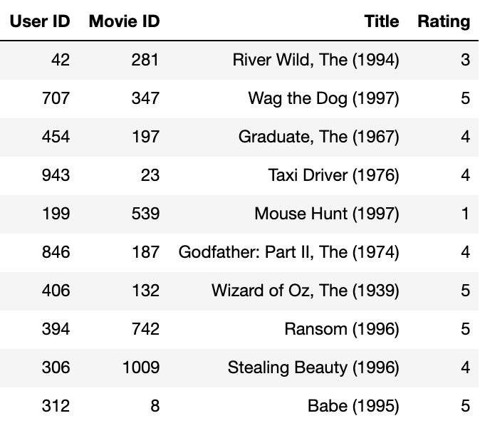
Every user is given a unique numeric ID (ranging from 1 to 943), and each movie is given a unique numeric ID too (ranging from 1 to 1682). User's ratings for movies are integers ranging from 1 to 5, with 5 being the highest.
Our objective here is to build a model that can predict how a user would rate a movie they haven't already seen, by looking at the movie ratings of other users with similar tastes.
If you want to follow along and run the code as you read, you can clone this notebook, install the required dependencies using conda, and start Jupyter by running the following commands on the terminal:
pip install jovian --upgrade # Install the jovian library
jovian clone 5bc23520933b4cc187cfe18e5dd7e2ed # Download notebook
cd movielens-fastai # Enter the created directory
jovian install # Install the dependencies
conda activate movielens-fastai # Activate virtual environment
jupyter notebook # Start Jupyter
Make sure you have conda installed before running the above commands. You can also click on the "Run on Binder" button at the top to start a Jupyter notebook server hosted on mybinder.org instantly.
You can download the MovieLens 100K dataset from this link. Once downloaded, unzip and extract the data into a directory ml-100k next to the Jupyter notebook. As described in the README, the file u.data contains the list of ratings.
On Linux and Mac, you can simply run the follwing cell to download and extract the data:
# Download and extract the data (only for Linux and Mac)
!rm -rf ml-100k ml-100k.zip
!wget -q http://files.grouplens.org/datasets/movielens/ml-100k.zip
!unzip -q ml-100k.zip
!ls ml-100k
README u.genre u.user u2.test u4.test ua.test
allbut.pl u.info u1.base u3.base u5.base ub.base
mku.sh u.item u1.test u3.test u5.test ub.test
u.data u.occupation u2.base u4.base ua.base
We begin the importing the required modules from Pandas and FastAI.
import pandas as pd
from fastai.collab import CollabDataBunch, collab_learner
We can now read the data from the CSV file u.data
into a Pandas data frame, and create a FastAI data bunch which:
cols = ['User ID','Movie ID','Rating','Timestamp']
ratings_df = pd.read_csv('ml-100k/u.data', delimiter='\t',
header=None, names=cols)
ratings_df.sample(5)
data = CollabDataBunch.from_df(ratings_df, valid_pct=0.1)
data.show_batch()
The model itself is quite simple. We represent each user u
and each movie m
by vector of a predefined length n
. The rating for the movie m
by the user u
, as predicted by the model is simply the dot product of the two vectors.
Here's a small subset of the users and movies, represented by randomly chosen vectors of length 5, and the predicted ratings:
Since the vectors are chosen randomly, it's quite unlikely that the ratings predicted by the model match the actual ratings. Our objective, while training the model, is to gradually adjust the elements inside the user & movie vectors so that predicted ratings get closer to the actual ratings.
We can use the collab_learner
method from fastai
to create a neural collaborative filtering model.
learn = collab_learner(data, n_factors=40, y_range=[0,5.5], wd=.1)
The actual model created here contains 2 important enhancements on the simpler version described earlier:
First, apart from the vectors for users and movies, it also add bias terms to account for outliers, since some users tend to always rate movies very high or very low, and some movies tend to be universally acclaimed or disliked.
Second, it applies the Sigmoid activation function to the above output, and scales it so that the result always lies in the given y_range
, which is 0 to 5.5 in this case.
The learner uses the mean squared error loss function to evaluate the predictions of the model, and the Adam optimizer to adjust the parameters (vectors and biases) using gradient descent. Before we train the model, we use the learning rate finder to select a good learning for the optimizer.
learn.lr_find()
learn.recorder.plot(skip_end=15)
LR Finder is complete, type {learner_name}.recorder.plot() to see the graph.
Upon inspection of the graph, we can see that the decrease in loss starts to decrease when the learning rate is around 0.01
. We can choose this as our learning rate, and train for 5 epochs, while annealing the learning rate using the 1-cycle policy, which leads to faster convergence.
learn.fit_one_cycle(5, 0.01)
In just 30 seconds, the mean squared error has come down to around 0.80, which is quite close to the state of the art (as compared with these benchmarks). And it only took us 8 lines of code to load the data and train the model!
While it's great to see the loss go down, let's look at some actual predictions of the model.
(users, items), ratings = next(iter(data.valid_dl))
preds = learn.model(users, items)
print('Real\tPred\tDifference')
for p in list(zip(ratings, preds))[:16]:
print('{}\t{:.1f}\t{:.1f}'.format(p[0],p[1],p[1]-p[0]))
Real Pred Difference
5.0 4.2 -0.8
4.0 3.2 -0.8
3.0 3.4 0.4
3.0 2.4 -0.6
3.0 2.9 -0.1
2.0 2.4 0.4
4.0 4.2 0.2
4.0 4.6 0.6
4.0 3.6 -0.4
1.0 2.3 1.3
5.0 4.3 -0.7
2.0 2.9 0.9
4.0 4.0 0.0
4.0 3.7 -0.3
5.0 4.4 -0.6
4.0 4.1 0.1
Indeed, the predictions are quite close to the actual ratings. We can now use this model to predict how users would rate movies they haven't seen, and recommend movies that have a high predicted rating.
As a final step, we can save and commit our work using the jovian
library.
!pip install jovian --upgrade -q
import jovian
jovian.commit()
[jovian] Saving notebook..
Jovian uploads the notebook to jvn.io, captures the Python environment and creates a sharable link for the notebook. You can use this link to share your work and let anyone reproduce it easily with the jovian clone
command. Jovian also includes a powerful commenting interface, so you (and others) can discuss & comment on specific parts of your notebook.
In a future post, we'll dive deeper and see how DataBunch
and collab_learner
are actually implemented, using PyTorch. We'll also explore how we can interpret the vectors and biases learned by the model, and see some interesting results.
In the meantime, following are some resources if you'd like to dive deeper into the topic:
Lesson 4 of FastAI's "Practical Deep Learning for Coders" course
Paper introducing neural collaborative filtering
PyTorch: Zero to GANs - tutorial series covering the basics of PyTorch and neural networks